Quantum Mechanics Notes

The Basics of Quantum Mechanics

Schrödinger

The Born Interpretation

ψ at a point x, has a probability for a particle being between x and x+dx proportional to |ψ|2dx. Therefore,

Ωψ = ωψ

Ω = eigenvalue and ψ = eigenfunction.

When not an eigenfunction, must be a superposition or more than one wave function.

Particle in a Box

Tunnelling – possibility of finding particle outside box classically forbidden.

Vibrational Motion

Rotational Motion

Spectroscopy

Hydrogenics

Spin Orbit Coupling

Electron has spin angular momentum, and this generates a magnetic field.

Spin + orbit interactions – j = l ± ½

Multiplicity = 2S + 1

Postulates of Quantum Mechanics

1a: the state of a system of N particles is fully described by a function ψ(r1, r2, … rN; t) – the wavefunction.

NOTES:

Spin omitted (for now).

1b: Born’s Probabilistic Interpretation.

The probability that a system in a state ψ will be found in the volume element dτ = dr1, dr2 .. drN is ψ*(r1 … rN, t) ψ(r1 … rN, t) dτ.

NOTES:

Statistical, even for 1 particle.

P(x,t) = | ψ(x,t) | 2 is the probability density.

Can deduce from here:

Normalisation –

Conserves probability.

Physically acceptable ψ:

• Single valued.
• Continuous.
• Finite.

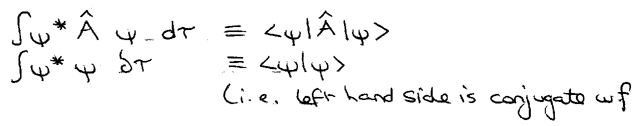
Dirac’s Bra-c-ket Notation –

2a: in quantum mechanics, observables are represented mathematically by operators: corresponding to every classical observable A there is a corresponding operator  which is linear and hermitian.

NOTES: e.g. x, px, E, etc.

3: Measurement. When a system is in a state described by ψ:

1. single measurement of an observable A always yields a single result – an eigenvalue an of Â.
2. Mean value of A equals the expectation value <Â>

Define Expectation Value:

                [ if ψ is normalised ]

Bra-c-ket:

<Â> = <ψ|Â|ψ> if <ψ|ψ> = 1.

NOTES:

From (i) – Probability Distribution:

Common Sense, as mean A = sum over all n of Pnan.

From (ii) – must expand ψ in terms of eigenfunctions of Â.

i.e. Pn = | cn | 2

Probability Pn that particular value an is measures is |cn|2, where cn is the coefficient of eigenfunction fn of  (in the expansion).

Dispersion in distribution of measurements is characterised by:

Root mean square deviation (RMS) ΔA =

(ΔA)2 = < (Â - <Â>)2> = < (Â2 - 2Â <Â> + <Â>2 ) >

(ΔA)2 = <Â2> - <Â>2

Special Case –

ψ is an eigenfunction of Â, so Âψ = aψ. < Â > is:

< Â > =

Pn = 1 or 0 (n=ε or n≠ε), then dispersion free – single measure value, aε. < Â > = aε, < Â2 > = aε2, ΔA = 0.

Thus, if ψ is an eigenfunction of  then observable A will always yield the same result.

2b: Choice of Operators.

OBSERVABLE	OPERATOR
Position, x
Linear momentum, px
Total Energy, E

All linear and hermitian.

Linearity –

Hermiticity –

 is Hermitian if:         < m |  | n > = < n |  | m >*

EXAMPLES:

The eigenvalues of Hermitian Operators are real:

Orthonormality –

The eigenfunctions for different eigenvalues of Hermitian Operators are orthogonal, i.e. if  | fn > = an | fn > and  | fm > = am | fm >, where am ≠ an, then < fm | fn > = 0.

Time Dependence and Stationary States

Classical Observable → Quantum Operator.

e.g. Kinetic Energy,

T = ½ m (px2 + py2 + pz2) →

Potential Energy,

V = V(x,y,z), so

Total Energy = T + V, → H(x,px)                [ Hamilton’s Function ]

Also note that the total energy operator from P2b is .

 - Time Dependent Schrodinger Equation, TDSE.

H is independent of time (in conservative systems), so always separable solutions to the TDSE of the form:

A system in a state described by this is said to be in a stationary state.

Its energy is a precise quantity (P3) and no measurable property of the system changes with time, i.e. <A>(t) = <A>(0) where <A>(t) is the expectation value of operator A at time t.

Proof:

NOTES:

This resolves the “radiation paradox” of old Quantum Mechanics. Stationary State → still not solved the TDSE. Need φn from TISE.

A common relation that is useful is:

To use this, it is necessary to understand what a commutator is.

Commutators, Complementary Observables,

and the Heisenberg Uncertainty Principle

ABf ≠ BAf in general, where A and B are operators.

Define:

Commutator [A,B] of A & B:

[A,B] = AB – BA

Compared the effects on a ghost function, e.g.

[x, px] f = (xpx – pxx) f                 = -ih (x(d/dx) – (d/dx)x) f        = -ih (x(df/dx) – (d/dx)(xf))        = ihf

Therefore [x,px] = ih.

If [A,B] = 0, they are said to commute. For example, [y,px] = 0 (independent x,y).

NOTES:

• [B,A] = - [A,B]
• [A,αB] = α[A,B]
• [A,B+C] = [A,B] + [A,C]
• [A,BC] = [A,B]C + B[A,C]

Uses:

From P3, Aψ = aψ and Bψ = bψ. This implies precise measurement of A and B, therefore [A,B] = 0 → precise value for each observable can be known simultaneously.

If [A,B] = 0, then there is an eigenfunction of A which is simultaneously an eigenfunction of B.

If [A,B] ≠ 0, it is NOT generally possible to measure the observables precisely and simultaneously.

These observables are said to be complementary or conjugate.

Heisenberg’s Uncertainty Principle:

ΔAΔB ≥ ½ | <[A,B] > |

Where,

(ΔA)2 = <Â2> - <Â>2

e.g. [x,px] = ih, → < [x,px] > = ih, so | < [x,px] > | = h

Hence, ΔxΔpx ≥ h/2

Applications of Quantum Mechanics

1 D free particle (no Potential)

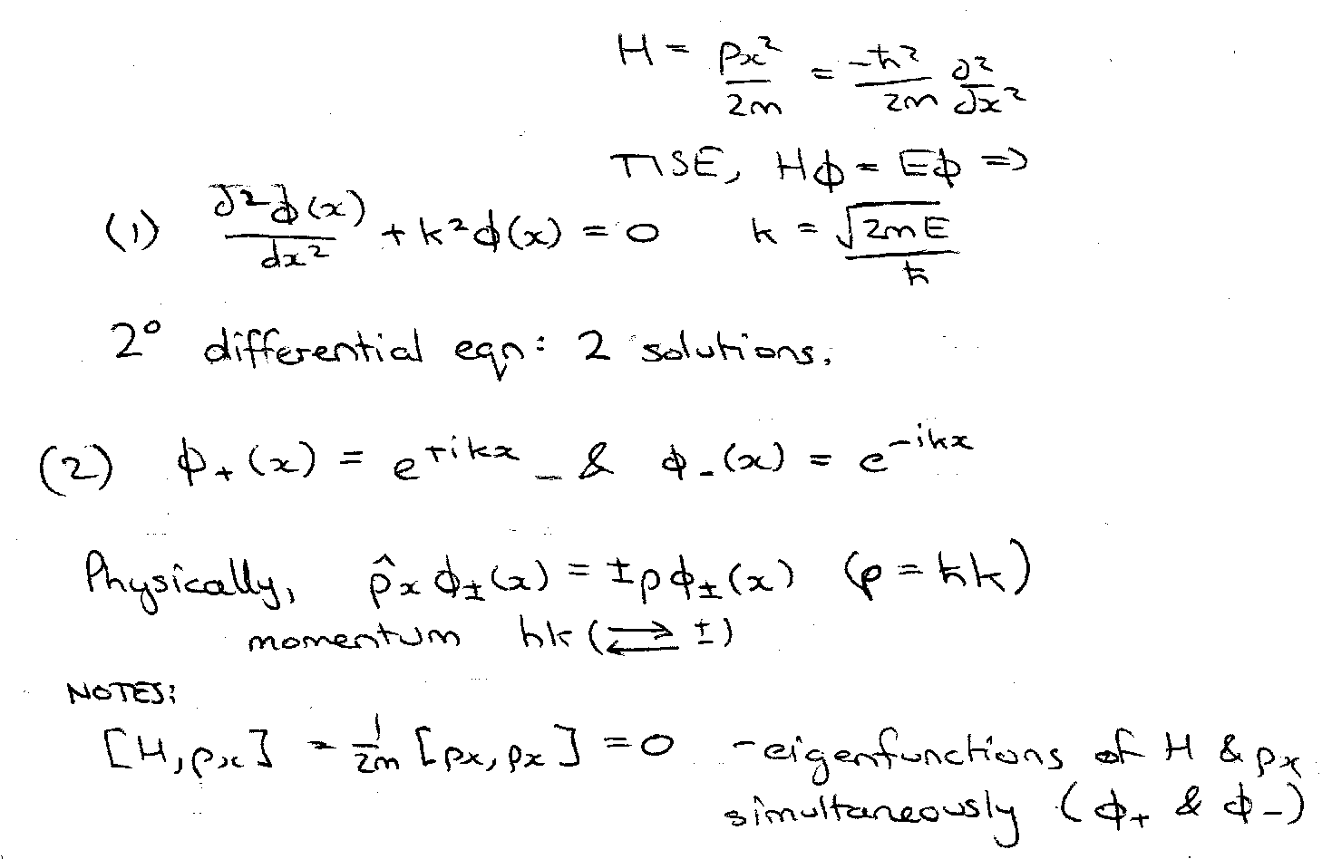
Note that general solution to (1) is a linear combination:

General interpretation using P3 is that there is always dispersion-free energy for the above, but the relative probability of finding the particle moving in a given direction with momentum ±hk is |A’|2|B’|2

General Solution to the Schrödinger Equation from the above (2) & (3):

Compare to classical standing waves,

cos (2πx/λ) + sin (2πx/λ)

Therefore 2π/λ = p/h , → λ = h/p                [ De Broglie Relation ]

Quantisation – Particle in a Box

Outside the Box: φ(x) = 0 – no particle here.

Inside the Box: V(x) = 0 so TISE same as free particle above. Solution as above is:

φ(x) = A cos (px/h) + B sin (px/h)

ψ(x) is continuous, therefore Boundary Condition: φ(0) = 0 = φ(L).

Hence,

φ(0) = 0 → A = 0.

φ(L) = 0 → B sin (pL/h) = 0.

Thus,

pL/h = nπ, where n = 1,2,3…

Also, p = √(2mE):

En = , n = 1,2,3…

Quantisation arose from the Boundary Condition. Quantum number n is established.

H φn(x) = En φn(x).

φn(x) = B sin (nπx/L) for 0 ≤ x ≤ L

φn(x) = 0 for x ≤ L, or x ≥ L

B, such that φn(x) is normalised, is found by:

Pictorially,

Probability Density | φn(x) | 2 → tends to classical limit (Correspondence Principle)

Energy Level Separation:

ΔE = En+1 – En =

So, ΔE → 0 as L → ∞

Extra Dimensions:

d = 2, En =

Lx = Ly → square box. n1 = n2 is single degenerate, while n1 ≠ n2 is doubly degenerate.

Degeneracy is a consequence of symmetry.

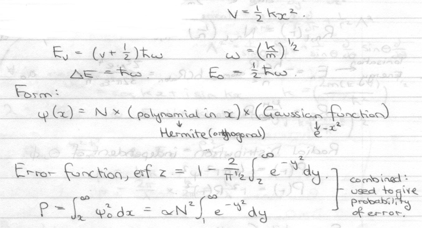
Harmonic Oscillator

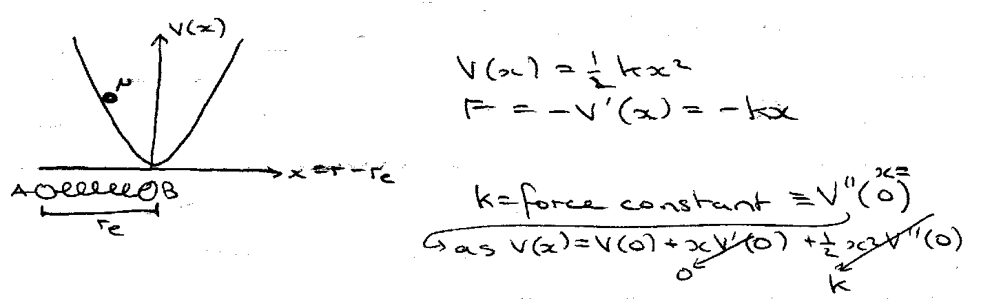
Classically, E = T + V = px2/2μ + ½ kx2

Quantum Mechanics:

E =

Satisfied for all x if both:

Normalise,

For remaining solutions try:

Pn(x) = polynomial in x.

Gives second order differential equations for Pn(x) when subbed into the Schrodinger Equation.

The solutions are called Hermite Polynomials.

Pn(x) = Hn (α x)

Eigenvalues En = (n+½)hω , n = 0,1,2…

Ho (α x) = 1                        [ even in x ]

H1 (α x) = 2α x                [ odd in x ]

H2 (α x) = 4αx2 – 2                [ even in x ]

… etc.

Hence,

Particle on a Ring

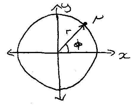
To get H:

Transform to polar cords.

Fix r, look at angular component of H.

Transforming to polar coordinates:

Fixing r means that & can be dropped. ψ = ψ(φ): dψ/dr = 0 = d2ψ/dr2.

Thus,

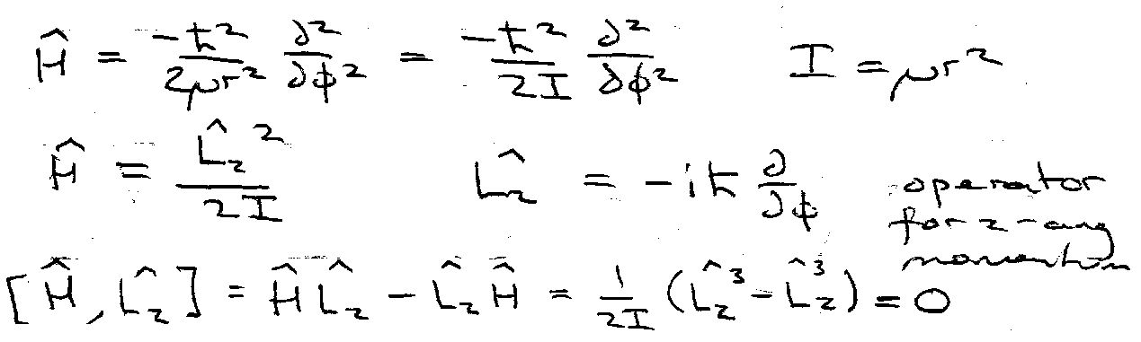
Therefore eigenfunctions of H can be chosen to be eigenfunctions of Lz.

Then,

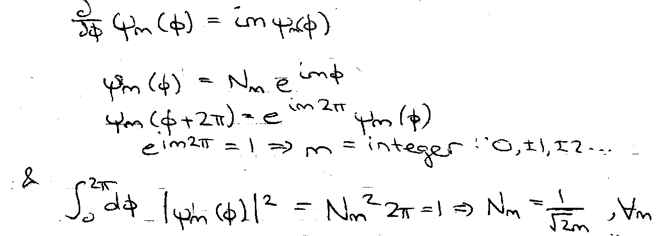
Therefore normalised eigenfunctions of H = which satisfy the boundary condition are:

NB: Em = is doubly degenerate for | m | > 0.

Particle on a Sphere

Transform to polar cords.

Consider angular parts.

Separate θ/φ dependence.

Separating variables,

Ordinary Differential Equation for (H)(θ), the Legendre Equation.

Solutions are associated Legendre functions,

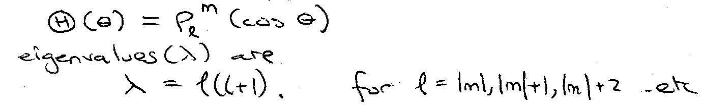
i.e. m = -l, -(l-1), … 0, … (l-1), l.

This gives the spherical harmonics:

Which satisfy:

Molecular Rotation

Equivalent to free motion of particle with reduced mass on surface of a sphere (radius re).

Therefore H =         [ J not L – convention for molecular systems ]

i.e. EJ = Bhc J(J+1)                [ rotational energy levels ]

B = h/(8π2Ic)                        [ units m-1 or cm-1 ]

J = 0,1,2 …

M = -J, -(J-1) … J.                [ projection of momentum along z ]

This is (2J+1) degenerate.

Atomic Orbitals

First, it is useful to refine our units onto the atomic scale:

In atomic units,

From (2) and (3), any atomic orbital can be written as separable:

This is the “associated Laguerre Equation”. En = -1/(2n2) Hartree, n = 1,2,3 …

Electron Spin

Stern & Gerlach (1922) passed beam of Ag atoms through an inhomogeneous magnetic field (i.e. a field gradient was present → force). Beam split in two.

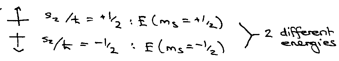
Ag (5s1). If S = ½, then ms = ± ½ … 2 components with different energies in a magnetic field.

1925 – splittings in atomic spectra. e- had intrinsic angular momentum of ½ h.

1930 – Dirac. Obtained wave equation for e- by combining Quantum Mechanics and Special Relativity. Equation predicted s = ½, confirming the above.

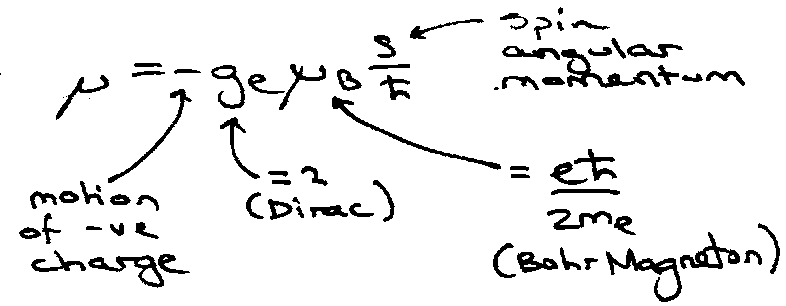
E = - μ . B

If B is in the z-direction, s.B = szBz, →

Spin Wavefunctions

Single electron:

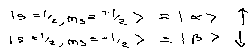
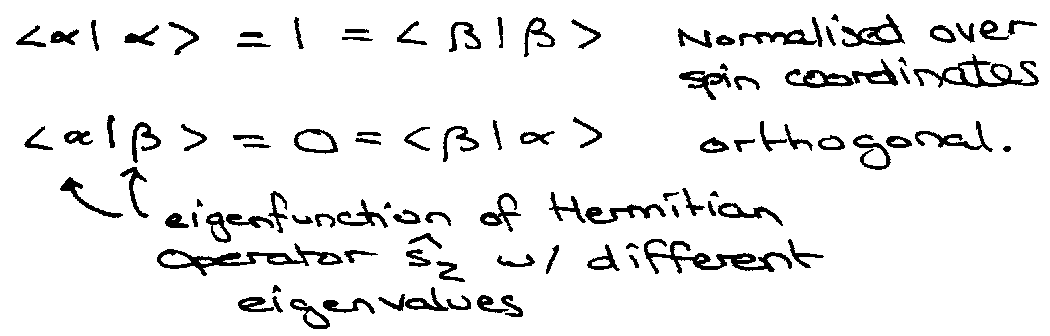
Satisfy usual angular momentum eigenvalue equations:

Also,

Two electrons:

Only linear combinations of following possibilities –

Possible values of Ms = m1 + m2 are:

Ms = 1,0,-1 (S=1) and Ms = 0 (S=0).

MS = S, S-1, .. –S → (2S+1) = 3 (triplet).

MS = S, S-1, .. –S → (2S+1) = 1 (singlet).

But what are corresponding 2 electron spin wavefunctions, | s, ms > ?

| S = 1, Ms = +1 > = | α1 α2 >

(as this is the only way to get Ms = +1).

Similarly,

| S = 1, Ms = -1 > = | β1 β2 >

(Ms = -1).

Both of these S=1 wavefunctions are symmetric wrt interchange of the 2 electrons (e1↔e2).

Hence, the remaining S=1, Ms=0 component of the triplet states must be symmetric too [ Ms quantum number depends on where we choose to put the z-axis, which clearly cannot affect the exchange symmetry of a triplet state ].

Hence, only possibility for:

| S = 1, Ms = 0 > = symmetric combination of , where the term outside the brackets is a Normalisation Constant.

Similarly,

| S = 0, Ms = 0 > = , which has antisymmetric exchange symmetry.

Pauli Exclusion Principle

Suppose quantum system contains two indistinguishable particles 1 and 2 such that:

ψ = ψ(1,2)

i.e. ψ is a function of all space and spin coordinates.

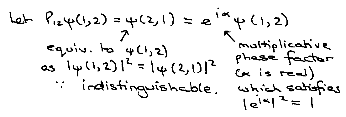
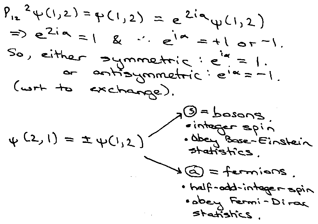
Repeat operation:

Corollary 1: Exclusion Principle in Orbital Space.

No 2 electrons can have the same set of 4 quantum number (n,l,ml,ms) within the orbital approximation.

Combination with the Aufbau Principle gives the Periodic Table.

Reason:

ψ(2,1) = ψn,l, ml, ms(2) ψn,l,ml,ms(1) = ψn,l, ml, ms(1) ψn,l,ml,ms(2) = +ψ(1,2)

But electrons are fermions so ψ(1,2) = -ψ(2,1).

Corollary 2: Exclusion Principle in Real Space.

2 electrons in a triplet state (S=1) cannot be at the same point in space.

ψ(1,2) = ψspace x ψspin

ψ(1,2) = ψ(r1,r2) x

Thus, ψspace must be antisymmetric wrt e1↔e2.

ψ(r2,r1) = - ψ(r1,r2)

Setting r2 = r1 = r:

ψ(r,r) = - ψ(r,r)

Therefore ψ(r,r) = 0 and | ψ(r,r) |2 = 0, so get a “Fermi Hole”.

Basis of Hund’s 1st Rule: triplet states are lower in energy than singlet states, all other things – including the electron configurations – being equal.

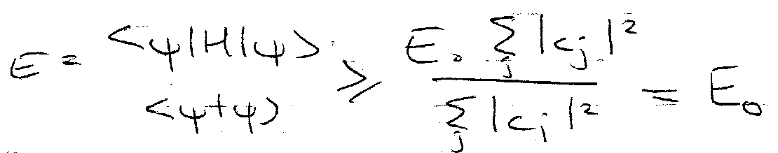
The Variational Method

How to find good approximate solutions to problems that can’t be solved exactly.

Where ψ = trial wavefunction and Eo = exact ground state energy.

So,

Suppose we have a trial wavefunction ψα that depends on a parameter α. Find the best α (most accurate wavefunction) by minimising:

Example – Quartic Oscillator

Similar to Harmonic Oscillator, so try that wavefunction as trial:

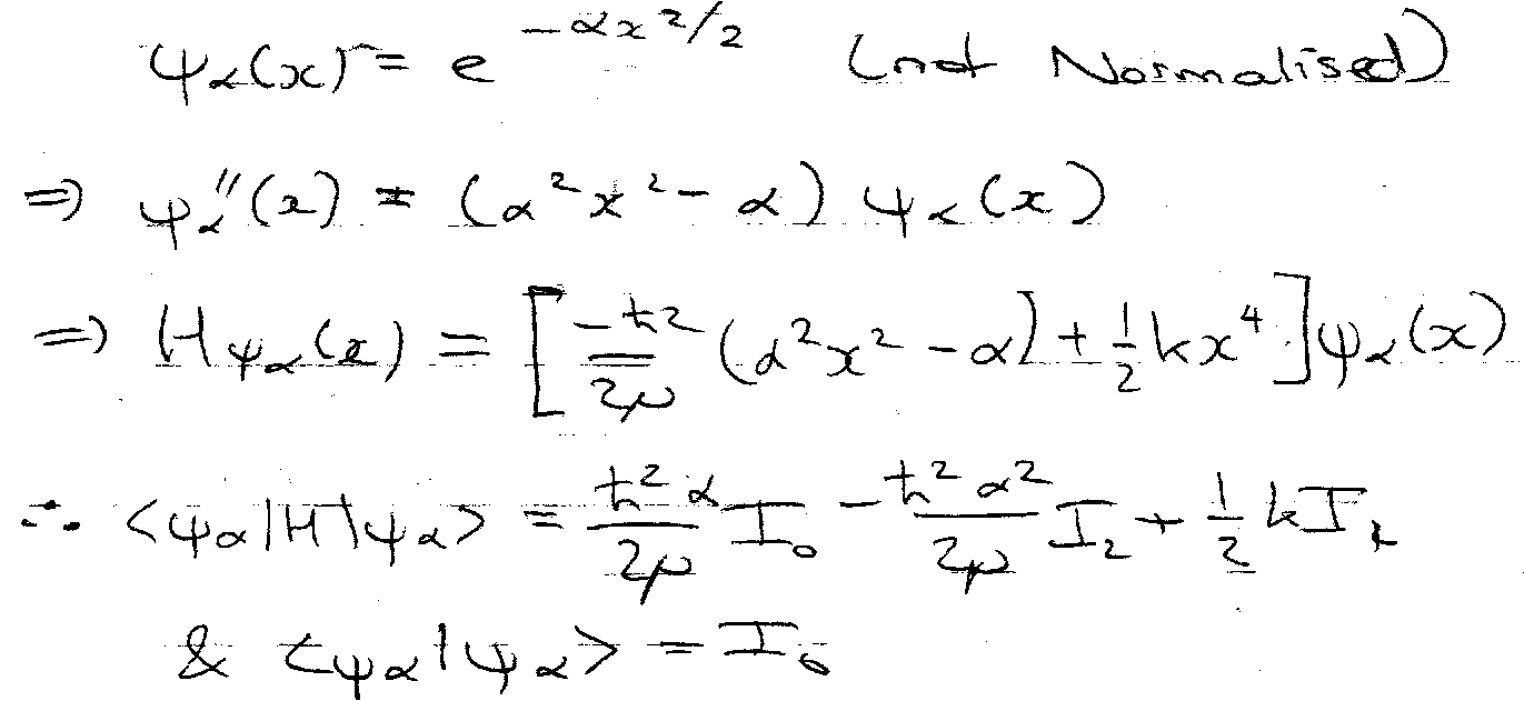
Where,

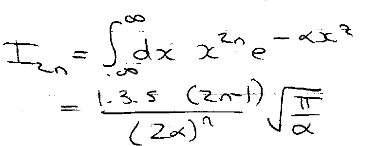
Hence,

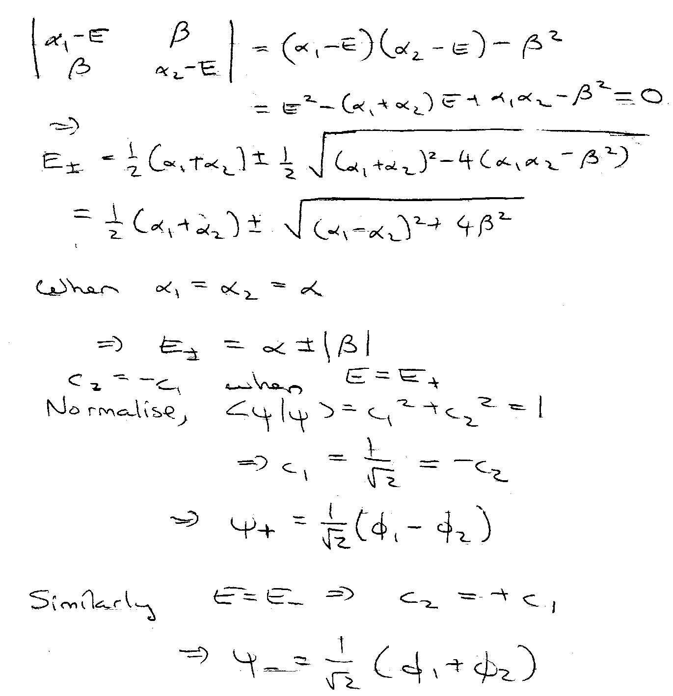
Example 2 – Secular Equations