Nuclear Magnetic Resonance Notes

When a magnetic nucleus is placed in a magnetic field, it adopts one of a small number of allowed orientations of different energy. For example, the nucleus of the hydrogen atom has just two permitted orientations. The magnetic moment can point in the same direction as the field, or in the opposite direction. These two states are separated by an energy ΔE, which depends on the strength of the interaction between the nucleus and the field, i.e. on the size of the nuclear magnetic moment and the strength of the magnetic field. ΔE can me measured by applying electromagnetic radiation of frequency v, which causes nuclei to flip from the lower energy level to the upper one, provided the resonance condition ΔE = hv is satisfied. This is nuclear magnetic resonance.

For a given field strength, the energy gap ΔE and therefore the resonance frequency, are determined principally by the nuclide observed, because every nuclide has a characteristic magnetic moment. But there is more to it than this. This is because the resonance frequency also depends slightly on the chemical environment of the nucleus in a molecule, an effect known as the chemical shift.

Angular Moment and Nuclear Magnetism

Spin Angular Momentum –

Magnetic nuclei possess an intrinsic angular momentum known as spin, whose magnitude is quantised in units of h/2π.

Magnitude of spin angular moment = [ I(I+1) ½ ] (h/2π)

The spin quantum number I of a nucleus may have one of the following values,

I = 0, 1/2, 1, 3/2, 2, …

With quantum numbers greater than 4 being rare. This number is determined largely by the number of unpaired protons and neutrons. For example, an isotope such as 12C has even numbers of protons and neutrons – all the protons pair up with antiparallel spins, as do all the neutrons, giving a net spin angular momentum of zero. A nucleus with odd numbers of protons and neutrons generally has an integral, non-zero quantum number because the total number of unpaired nucleons is even, and each of the contributes a half to the quantum number. However, it is difficult to predict exactly how many protons and neutrons will be unpaired except in cases such as 2H.

Space Quantisation –

Spin angular momentum is a vector quantity – its direction as well as its magnitude is quantised. The angular momentum I (not to be confused with the quantum number I) of a spin-I nucleus has 2I+1 projections onto an arbitrarily chosen axis, say the z-axis. Hence, the z component of I, denoted Iz is quantised:

Iz = mh

Where m (magnetic quantum number) has 2I+1 integral values between +I and –I.

Nuclear Magnetisation –

The magnetic moment of a nucleus is intimately connected with its spin angular momentum. To be more precise, the magnetic moment μ (also a vector quantity) is directly proportional to I with a proportionality constant γ, known as the gyromagnetic ratio.

μ = γI.

(The magnetic moment of a nucleus is not simply the sum of the magnetic moments of the constituent protons and neutrons).

Effect of a magnetic field –

In the absence of a magnetic field, all 2I+1 orientations of a spin-I nucleus have the same energy. This degeneracy is removed when a magnetic field is applied – the energy of a magnetic moment μ in a magnetic field B is minus the scalar product of the two vectors –

E = - μ.B

In the presence of a strong field, the quantisation axis z is no longer arbitrary, but coincides with the field direction. Therefore,

E = - μzB

Combining this with the above we can write:

E = – m h γ B

That is, the energy of the nucleus is shifted by an amount proportional to the magnetic field strength, to the gyromagnetic ratio and the z component of the angular moment. The 2I + 1 states for a spin-I nucleus are equally spaced, with energy gap hγB.

The selection rule for NMR is Δm = ±1. The allowed transitions are therefore between adjacent energy levels. The resonance condition ΔE = hv is thus:

ΔE = hv = h γ B

or,

v = γB / 2π

where v is the frequency of the electromagnetic radiation. All 2I allowed transitions for a spin-I nucleus have the same energy.

The magnetic field experienced by a nucleus in a molecule differs slightly from the external field such that the exact resonance frequency is characteristic of the chemical environment of the nucleus. This interaction is the chemical shift.

NMR Spectroscopy

Resonance frequencies –

A typical magnetic field strength used for NMR is 9.4T, roughly 105 times stronger than the earth’s magnetic field. For hydrogen nuclei, it is predicted that the resonance frequency will be 400MHz. This falls in the radio frequency region of the electromagnetic spectrum and corresponds to a wavelength of 75cm. The radiation required to induce NMR transitions is consequently referred to as the radiofrequency field. Magnetic fields in the range 1.4-14.1T are commonly used, giving proton resonance frequencies of 60-600MHz. Hydrogen has the largest gyromagnetic ratio (and the largest magnetic moment) with the exception of 3H (Tritium).

Populations of Energy Levels –

When placed in a magnetic field, a collection of magnetic nuclei spread themselves amongst the 2I+1 available energy levels according to the Boltzmann distribution. Considering protons in a 9.4T field at 300K, the ratio of populations of the two levels is,

Where ΔE, the energy gap, equals hγB. Evaluating this expression, ΔE = 2.65x10-25J, while kT = 4.14x10-21J. Clearly, the energy required to reorient the spins is dwarfed by the thermal energy kT, so that there will be very little tendency for the spins to become ordered in the lower energy level. With such small values of ΔE/kT, it is possible to simplify the equation above to obtain the normalised population difference:

With the above numbers, this gives a population difference of 3.2x10-5, or one part in about 32000. This difference will be even smaller for protons in a weaker field, or for nuclei with lower gyromagnetic ratios. This situations is in stark contrast to electronic spectroscopy at a frequency of, say, 6x1016Hz. Here ΔE is much larger than kT and almost all of the molecules will be in their ground state, leaving the excited state virtually empty.

In any form of spectroscopy, an electromagnetic field excites molecules or atoms or electrons or nuclei as the case may be, from the lower energy level to the upper one with the same probability as it induces the reverse transition. The net absorption of energy and hence the intensity of the spectroscopic transition is therefore dependent on the difference in populations of the two levels. In NMR spectroscopy, where the upwards transitions outnumber the downward transitions by only one in 104-106, it is as if one detects only one nucleus in every 104-106. Add to this the fact that spectroscopy at higher frequencies is much more sensitive as a rule, because higher energy photons are easier to detect, and it becomes clear that NMR signals must be rather weak. It is therefore of crucial importance to optimise signal strengths, for example by using strong magnetic fields to maximise ΔE. Similarly, nuclei with large gyromagnetic ratio and high natural abundance are favoured.

Spin-spin Coupling

The chemical shift is not the only source of information encoded in an NMR spectrum. Magnetic interactions between nuclei give rise to extra NMR lines which give valuable clues to the arrangement of atoms in molecules.

Widths of NMR lines –

The NMR lines of many nuclei are exceedingly narrow: it is relatively straightforward on a modern spectrometer to resolve two resonances that differ in frequency by only one part in 109 (typical linewidths in 1H spectra of small molecules in solution are around 0.1Hz). This very high resolution comes about because nuclear magnetic moments are very weak, and interact very weakly with their surroundings. Not all nuclei will give sharp lines however. This is typically the case for nuclei with spin quantum numbers greater than ½.

Chemical Shifts

Nuclear Shielding –

These arise because the field, B, actually experienced by a nucleus in an atom or molecule differs slightly from the external field, B0 i.e. the field that would be felt by a bare nucleus, stripped of its electrons. In an atom, B is slightly smaller than B0 because the external field causes the electrons to circulate within their atomic orbitals. This induced motion, much like an electric current passing through a wire, generates a small magnetic field B’ in the opposite direction to B0. The nucleus is thus shielded from the external field by its surrounding electrons (B = Bo – B’).

B’ is proportional to B0 (the stronger the external field, the more effect it has on electrons). The field at the nucleus is typically written as:

B = B0 (1-σ)

Where σ, the constant of proportionality between B’ and B0, is called the shielding constant. As a result of nuclear shielding, the resonance condition becomes:

i.e. the resonance frequency of a nucleus in an atom is slightly lower than that of a bare nucleus.

Similar effects occur for nuclei in molecules, except that the motion of the electrons is rather more complicated than in atoms, and the induced fields may either augment or oppose the external field. Nevertheless, the effect is still referred to as nuclear shielding. Both the size and sign of the shielding constant are determined by the electronic structure of the molecule in the vicinity of the nucleus. The resonance frequency of a nucleus is therefore characteristic of its environment.

Measuring Chemical Shifts –

The shielding constant σ is an inconvenient measure of the chemical shift. Since absolute shifts are rarely needed and difficult to determine, it is common practice to define the chemical shift in terms of the difference in resonance frequencies between the nucleus of interest (v) and a reference nucleus (vref) by means of a dimensionless parameter δ:

The frequency difference v-vref is divided by vref so that δ is a molecular property, independent of the magnetic field used to measure it. The factor of 106 simply scales the numerical value to a more convenient size (quoted in parts per million).

This can be rewritten in terms of σ as:

Where σref << 1 has been used. An increase in σ (greater shielding) leads to a decrease in δ: δ is thus a deshielding parameter.

The reference signal is most conveniently obtained by adding a small amount of a suitable compound to the sample. For 1H and 13C this is usually tetramethylsilane, due to its solubility and strong 1H resonance from its 12 identical protons. Also the nuclei are strongly shielded so the resonance falls at the low frequency end of the spectrum (making most chemical shifts conveniently positive).

Note that changing the frequency of the spectrometer will not change the chemical shift (as it is unitless), but the resonance frequency relative to the reference is reduced in proportion to B0 (so for a spectrometer frequency half the size, the resonance frequency of the environment will also half).

Origin of Chemical Shifts

A magnetic field can induce two kinds of electronic current in a molecule – diamagnetic (opposes external field) and paramagnetic (augments external field). Diamagnetic and paramagnetic currents flow in opposite directions and give rise to nuclear shielding and deshielding respectively. The shielding constant may thus be written as a sum of diamagnetic (σd – positive) and paramagnetic (σp – negative) contributions.

Diamagnetic currents arise from the movement of electrons within atomic or molecular orbitals. The external field causes electrons to circulate in a plane perpendicular to the field direction. The current so induced generates a small local field opposed to B0. The magnitude of the diamagnetic current is determined solely by the ground state electronic wavefunction of the atom or molecule, depends sensitively on the electron density close to the nucleus and provides the only contribution to σ for spherical, closed-shell atoms. The diamagnetic shielding is fairly easy to calculate for atoms and varies strongly with the number of electrons.

Paramagnetic currents also arise from the movement of electrons within molecules, but by a more circuitous route. Imagine a somewhat artificial molecule with just two electronic states – a ground state with the form of an atomic px orbital containing two electrons with paired spins, and an unoccupied excited state resembling a py orbital. An external magnetic field applied along the z axis distorts the wavefunction of the ground state by mixing it into a small fraction of the excited state wavefunction. In this way, the field partially overcomes the energy gap between px and py, which keeps the electrons locked along the x axis, and creates a path for electrons to circulate in the xy plane. This induced current generates a magnetic field which (it turns out) augments the external field and deshields a nucleus at the centre of the electron density.

The extent of deshielding is clearly linked to the energy gaps involved – other things being equal, low-lying excited states should make a greater contribution than higher energy states. Theory suggest that σp should be approximately inversely proportional to the average excitation energy. The paramagnetic shift is also related to the distance R between the nucleus and its surrounding electrons (R-3).

Contributions to Nuclear Shielding

Almost impossible to be able to calculate chemical shifts from first principles, as need a large amount of information on all the wavefunctions. Simplest to consider the contributions to σ as one of four parts:

1. Local diamagnetic shielding
2. Local paramagnetic shielding
3. Shielding due to remote currents
4. Other sources of shielding

The first two are contributions from electrons in the immediate vicinity of the nucleus. The third accounts for electrons circulating around other nearby nuclei. The final part includes electric field shifts, H-bonding, solvent shifts, unpaired electrons, etc.

Local Diamagnetic Shifts –

Strongly dependent on electron density around the nucleus. The larger the electron density, the greater the shielding and the smaller the chemical shift. This is aptly shown by methyl halides, where increasing electronegativity of the halogen leads to electron-withdrawal from the methyl group, deshielding the protons. This effect is relatively short range, e.g. on 1-chlorobutane, C1 is strongly affected, C2 and C3 only slightly, and C4 negligibly.

Local Paramagnetic Shifts –

Dependent on ΔE and R-3 as mentioned. The former is well illustrated by transition metal complexes (field splitting). The latter is well shown by monosubstituted benzenes (13C) – e-donation to ortho and para carbons leads to increased electron repulsions at these orbitals, so they expand (reduces R-3 and hence δ).

Neighbouring Groups –

The best example of this is benzene, although it is common in acetylene derivatives. For example, looking at the trend for acetylene, ethylene and ethene. Based on hybridisation and consequent s-character we expect chemical shift to decrease along this series. However, π-electrons cause shielding and the neighbouring group effect of the C=C bond deshields the protons.

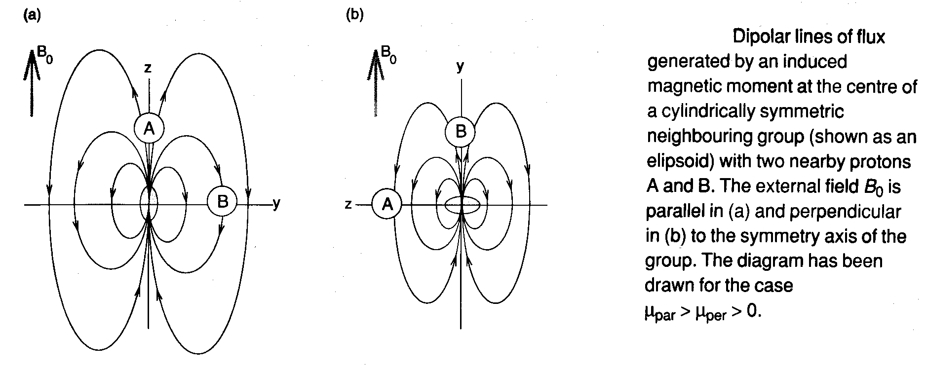
In aromatic compounds, the extensive π-electron clouds supports large electronic currents. The dominant contribution to the magnetic anisotropy comes from the circulation of these electrons within their delocalised molecular orbitals, i.e. the neighbouring group effect is due principally to the diamagnetic moment induced when the external field is perpendicular to the molecular plane (right).

However, the end result is the same as acetylene because the induced diamagnetic moment is opposed to the external field so that the anisotropy is negative. Thus, we can anticipate deshielding for nuclei in the plane of the aromatic ring, and shielding for any nuclei above or below the ring.

This ring current shift is demonstrated clearly by benzene itself, whose 1H shift is 1.4ppm to the high frequency side of the olefinic protons in cyclohexa-1,3-diene. A more interesting example is the dimethyl substituted pyrene, which with 14π electrons, is aromatic according to the 4n+2 rule. The ring protons are deshielded, as expected, but the methyl groups, which protrude above and below the plane of the molecule, are shielded by more than 5ppm relative to ethane. These protons lie in a region where the induced field opposes the external field.

Similarly, planar annulene with 4n+2 = 18 shows two proton resonances, one from the 12 strongly deshielded external protons, and one at -3ppm from the 6 internal protons. The latter set of Hs lie within the current loop formed by the circulating π-electrons, and are shielded by the ring current.

The magnitude of the neighbouring group effect depends on the magnetic anisotropy of the group itself and not on the nucleus. Hence this is relatively more important for protons (due to their small local diamagnetic and paramagnetic shielding effects).

Other sources of chemical shifts –

Hydrogen bonding is responsible for some of the largest observed deshielding effects in 1H NMR. The hydrogen-bonded proton is heavily deshielded. This effect is stronger for intramolecular H-bonds (as they are usually stronger).

Chemical shifts are also affected by the local electric fields arising from charged or polar groups. These can modify diamagnetic and paramagnetic currents by polarising local electron distributions, and by perturbing ground and excited state wavefunctions and energies. Positive charges usually deshield nearby protons, while negative charges often cause shielding.

There are also paramagnetic shifts produced by unpaired electrons (referring to the magnetic moment of the electron and not to the induced electronic currents discussed above). Unpaired electrons give rise to large dipolar magnetic fields – the gyromagnetic ratio of the electron is 660 times that of the proton.

Spin-Spin Coupling

Magnetic interaction between nuclei can also be used to elucidate structure. This nuclear spin-spin coupling causes NMR lines to split into a small number of components with characteristic relative intensities and spacings.

For example, in H13CO2-, we see two lines (a doublet) in each of the 1H and 13C NMR spectra. The splitting gives the strength of 1H-13C spin-spin interaction and is the same in the two spectra.

The 1H resonance is split into two because the magnetic moment of the 13C nucleus is the source of a small local magnetic field whose direction is determined by the 13C magnetic quantum number. When the 13C is its in m=+½ state, its magnetic field at the position of the 1H opposes the external field and shifts the 1H resonance to lower frequency. Conversely, for m=-½ carbon, the local field adds to the external field at the proton and moves its resonance to a higher frequency. Hence, two lines are seen.

Since the difference in energy between the two configurations of the carbon nucleus is tiny compared to the thermal energy, the two values are equally likely and the two components of the 1H doublet are equally intense. An exactly analogous argument explains the splitting of the 13C resonance by the 1H. It should be noted that homonuclear couplings, e.g. between protons with different chemical shifts, give rise to splittings in exactly the same way.

The properties of spin-spin coupling may be summarised and generalised in the following simple expression for the energy of two interacting nuclei A and X (not necessarily spin-½ either):

E = hJAXmAmX

In which mA and mX are the magnetic quantum numbers of the two nuclei and JAX is the spin-spin coupling constant. The latter is measured in Hz and may be positive or negative – if the antiparallel arrangement of nuclear spins is energetically favoured then it is positive, while if parallel spin is lower in energy it is negative (although this will have no effect on the appearance of the spectrum).

Combining this equation with the NMR selection rule, it can be seen that AX interaction shifts the NMR frequency of spin A by an amount -JAXmX. This leads to the general resonance condition for spin A:

where the summation runs over all spins (X) with appreciable spin-spin coupling to A.

Note that the allowed transitions are those in which a single spin flips.

Multiplet Patterns

Assuming all spin pairs are weakly coupled (difference in frequencies greatly exceeds their coupling), and all are spin-½ unless stated. Consider the effect of nuclei M and X on the NMR signal of nucleus A. Convention dictates that spins with very different chemical shifts are labelled by letters far apart in the alphabet. Nuclei with similar shifts are likely to be strongly coupled.

Coupling to a single spin-1/2 nucleus (AX) –

This is the H13CO2- example as already discussed – two equally intense lines centred at the chemical shift of A.

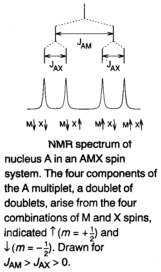
Coupling to two inequivalent spin-1/2 nuclei (AMX) –

Three nuclei with different chemical shifts and three distinct coupling constants. This is best analysed using the diagram on the left.

Hence, four lines are expected because there are four non-degenerate arrangements of the M and X spins. These peaks are displaced from the chemical shift of A by simple combinations of the couplings to spin A. This is known as a doublet of doublets.

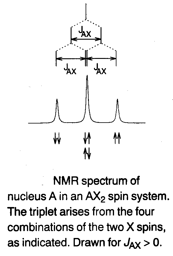
Coupling to two equivalent spin-1/2 nuclei (AX2) –

Special case of the AMX system, where JAM = JAX. The two central lines of the doublet of doublets coincide to give a triplet centred at the chemical shift of A, with the line-spacing equal to the coupling constant, and relative intensities 1:2:1 (see right).

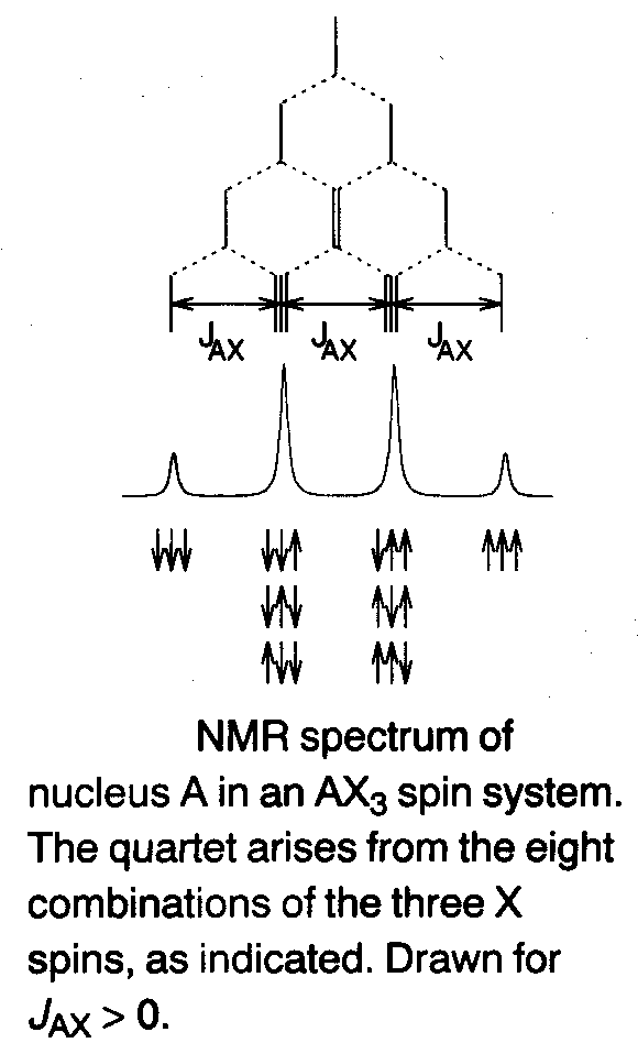
Coupling to three equivalent spin-1/2 nuclei (AX3) –

The multiplet pattern of A in an AX3 spin system is a four line quartet (see left).

Coupling to n equivalent spin-1/2 nuclei (AXn) –

It should now be clear how to generalise the above results. For n equivalent spin-½ nuclei, the A resonance is split into n+1 equally spaced lines, with relative intensities given by simple combinatorial arithmetic. The amplitude of the mth line (m=0,1,2,…n) of an AXn multiplet is simply the number of ways of finding m spins up and the remainder down, i.e. n!m!(n-m)!. To put it another way, the amplitudes are given by the coefficients in the binomial expansion of (1+x)n or equivalently by the (n+1)th row of Pascal’s Triangle.

Coupling involving I > ½ Nuclei –

If the nucleus of interest, A, has spin quantum number greater than ½, the multiplet structure can be predicted in exactly the same way as for spin-1/2 nucleus. For example, 14N (I=1) and 15N (I=½) NMR spectra of, respectively, 14NH4+ and 15NH4+ both consist of a quintet, with relative peak intensities 1:4:6:4:1. The NH coupling constants of the two isotopomers are in the ratio 0.73:1, which is the ratio of gyromagnetic ratios of the two nitrogen isotopes.

However, nuclei with I>½ possess, in addition to their magnetic dipole moment, an electric quadrupole moment that can interact with local electric field gradients. For molecules tumbling in solution, this interaction can lead to efficient relaxation of the quadrupolar nucleus and NMR lines that are so broad that the expected multiplet patterns are partially or completely obscured.

For A (I=½) coupled to X (I>½) the principles above can easily be extended. The magnetic moment of a spin-I particle has 2I+1 orientations with respect to the magnetic field B0. Therefore a nucleus coupled to a single X spin with quantum number I should show a multiplet comprising 2I+1 lines with equal spacings and amplitudes. For example, the 13C spectrum of deuterated chloroform, 13CDCl3 is a 1:1:1 triplet arising from the three equally probable states of the deuteron, m = +1,0,-1. Once again, quadrupolar relaxation may upset these predictions. Rapid relaxation of the quadrupolar nucleus may have the effect of decoupling A and X, such that no splitting is observed in the spectrum of A. For example, 35Cl and 37l (both I = 3/2) rarely produce splittings in the NMR spectra of nearby nuclei.

For coupling to equivalent I > ½ nuclei, the multiplet patterns are easily deduced using the tree diagram approach. For instance, the terminal protons of 11B2H6 show a 1:1:1:1 quartet due to coupling to the directly bonded 11B (I=3/2), while the bridge protons exhibit a seven line pattern with relative intensities 1:2:3:4:3:2:1, arising from equal interactions with the two symmetrically placed borons.

Equivalent Nuclei

There are in fact two kinds of equivalence – chemical and magnetic. Using examples of CH2F2 and CH2=CF2 and their coupling to the two fluorines Fa and Fb. In CH2F2 the two protons have the same chemical shift and each has identical couplings to Fa and Fb – as such they are termed magnetically equivalent. The same cannot be said of CH2=CF2, where the cis and trans 1H-19F coupling constants differ – in this case the protons are said to be chemically equivalent.

More generally, a set of nuclei with identical chemical shifts (call them a,b,c…) are magnetically equivalent if, for every other nucleus (e.g. z) in the molecule, the spin-spin coupling constant satisfy the relation:

Jaz = Jbz = Jcz

 As might be expected, the NMR spectra of molecules containing chemically equivalent spins are rather more complex than for similar compounds with magnetically equivalent nuclei. For example, the 1H spectrum of CH2=CF2 has no fewer than 10 lines. The analysis of such spectra is not straightforward!

The 1H spectrum of CH2F2 comprises just three lines, a 1:2:1 triplet with splitting equal to the proton-fluorine coupling constant. The remarkable thing about this spectrum is not the triplet, but the absence of any splittings arising from the proton-proton coupling. Although the two protons interact with one another, this coupling does not manifest itself as a splitting in the spectrum. In fact this is a general feature of scalar coupling – spin-spin interactions within a group of magnetically equivalent nuclei do not produce multiplet splittings. This is actually because of the changes in transition probabilities and NMR frequencies arising from the mixing of spin states by the spin-spin interaction.

Strong Coupling

This falls in between spin-spin coupling (change in frequencies much greater than J – weak coupling) and equivalent frequencies. For a range δν values:

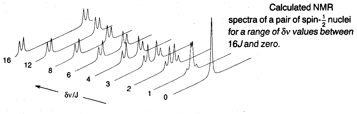
This is for a pair of spin-½ nuclei. As the difference in resonance frequencies is reduced, keeping J fixed, the inner component of each doublet steadily increases in amplitude, while the outer components become weaker. The two doublets move together as their chemical shift difference vanishes, until at δν = 0 the inner lines coincide and the outer lines vanish.

This occurs because the effect of the scalar coupling is to mix the spin states, so modifying their wavefunctions and energies. The result is a change in the transition probabilities of the four NMR lines, the inner lines becoming more allowed (i.e. stronger) and the outer pair less so (weaker). The effect is more pronounced the smaller the gap δν is between the nearly equivalent nuclear spin wavefunctions relative to J.

This gets consider more complicated for three or more nuclei, and masks the information likely to be extracted. Fortunately the problem of strong coupling is diminished easily, because coupling constants are independent of the static magnetic field while δν is not. Thus a strongly coupled spin system can often be made weakly coupled by using a higher field spectrometer.

Properties of Scalar Coupling

The strength of the interaction is crucially dependent on the s-electron character of the ground state and electronically excited state wavefunctions at the positions of the nuclei. The coupling is not affected by the strength or the direction of the external magnetic field, in contrast to the differences in resonance frequencies that arise from nuclear shielding. Indirect spin-spin couplings are therefore independent of the spectrometer frequency, and being isotropic are not affected by molecular tumbling.

One-bond and Two-bond Couplings

The interpretation of the magnitudes of scalar coupling constants is, in most cases, even more of a problem than it is for chemical shifts, and not one that will be tackled easily.

One-bond carbon-proton couplings 1JCH generally fall in the range 100-250Hz, and are sensitive to the s-electron character of the carbon atomic orbital involved in the bond, reflecting the crucial role played by the contact interaction.

Two-bond (geminal) proton-proton couplings vary over a wide range (-23 to +42 Hz) with large substituent effects – sp2 hybridised CH2 groups generally have smaller 2JHH than methyls.

Three-bond couplings

These coupling constants are found to vary with the dihedral angle between the two H-C-C- planes in H-C-C-H according to the Karplus relation:

3J = A + B cos θ + C cos2 θ.

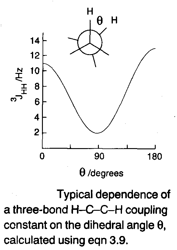
Although it is possible to calculate approximate values for A, B and C, it is more common to treat them empirically using conformationally rigid model compounds of known structure. Typical values are A = 2Hz, B = -1Hz, C = 10Hz which gives the shape of the curve above (Karplus Curve).

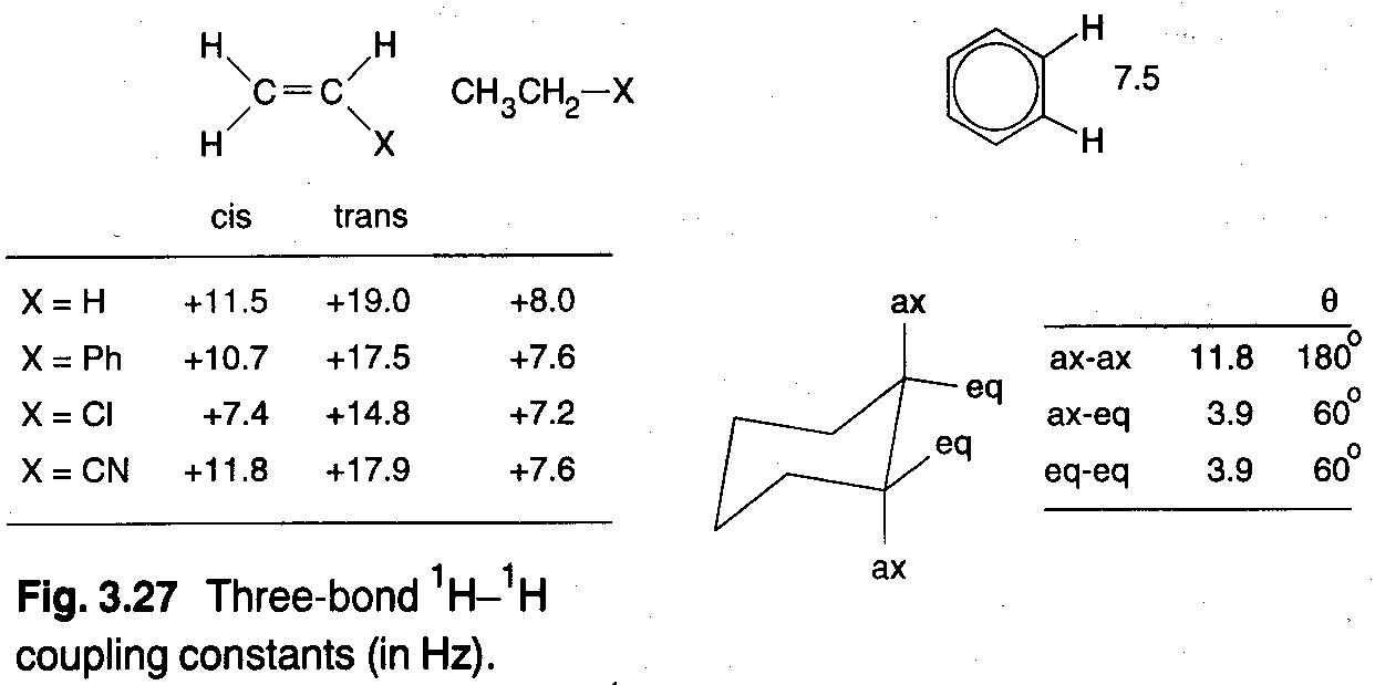
The utility of three-bond couplings lies principally in conformational analysis – 3JHH values for the ring protons in cyclohexanes depend on axial/equatorial protons, and the trans proton coupling constants across a C=C bond are up to a factor of 2 larger than the cis couplings.

It is also particularly useful in studies of protein structures (amide protons – helices and sheets).

Long-range Couplings

Proton-proton coupling constants are generally very small (< 1Hz) when the nuclei are separated by more than three bonds. A few of the exceptions are:

Chemical Exchange

Turning now to the processes capable of removing, or at least modifying, some of the NMR spectrum’s structure – namely dynamic equilibria. Consider a molecule converting between two conformations of equal energy:

A ⇌ B

With identical forward and backward first order rate constants, k. A good example is dimethylnitrosamine (Me2NNO). The skeleton of the molecule is planar due to partial double-bond character of the N-N bond, but it is not rigid. The nitroso group can undergo 180o rotations, so interconverting between two degenerate forms. At low temperatures, the internal rotation is slow and the 1H spectrum comprises two equally intense resonance from the methyl groups cis and trans to the oxygen. At higher temperatures, the nitroso group flips at an appreciable rate, and every time it does so, the chemical shifts of the two sets of protons switch back and forth, with an average time between jumps of τ = 1/k. This is chemical exchange (note that it may or may not involve making/breaking bonds).

Symmetrical Two-Site Exchange

This is as above, with equal forward and backward rates. A pattern like the following is usually observed over a range of rate constants:

Several questions immediately arise from this. Why are the two lines broadened by slow exchange? Who do they merge into a single sharp line when exchange is fast, rather continuing to get broader? Why does the rate have to be large compared to the difference in frequencies to average the two environments?

Slow Exchange –

This is the regime in which the separate resonances are exchange-broadened but are still to be found at frequencies vA and vB. At this limit, the increase in linewidth as a result of exchange is simply given by:

Where Δv is defined by the diagram on the left.

i.e. the faster the exchange, the wider the line. The origin of this effect is lifetime broadening, sometimes called uncertainty broadening because of its loose connection with Heisenberg’s Uncertainty Principle. The energy of a state of finite lifetime cannot be specified precisely – the shorter lived the transitions between such ‘blurred’ energy levels result in broadened spectroscopic lines. It is for this reason that electronic transitions have larger natural linewidths than rotational or vibrational spectra (faster spontaneous emission).

Fast Exchange –

The other extreme, in which the two lines have merged to form a single broadened resonance at the mean resonance frequency, is termed fast exchange. In this limit, the extra linewidth due to chemical exchange is:

, where δν = νA - νB

In contrast to slow exchange, where separate resonances are broadened by site-hopping, the single line observed in fast exchange becomes narrower as rate increases, reflecting the more effective averaging of the two environments A and B. That is, fast exchange causes the spins to experience an effective local field that is the mean of the two sites between which they hop.

To be able to detect separate signals from the two sites, they must acquire an appreciable phase difference, say 180o, which takes a time ½(δν)-1 (assuming vA > vB). If exchange occurs during this period, the accumulation of the phase difference is interrupted. When the spins swap frequencies, δν changes sign, and the phase difference starts to decrease. When the spins jump back to their original frequencies, their phase difference increases once more. So, the phase difference undergoes a random walk with frequent reversals.

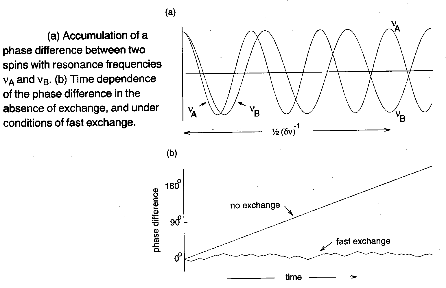
The result, in the fast exchange regime, is a root-mean-square phase difference at the end of the ½(δν)-1 period that is much smaller than 180o so that, in effect, the two signals have very similar frequencies. In other words, fast exchange destroys the frequency difference vA – vB, provided the rate of site-hopping k is much faster than the build-up of the phase difference (rate ≈ δν). The resonance observed in the fast exchange limit appears at the mean frequency ½ (vA + vB), because each spin spends, on average, 50% of its time in each site.

Intermediate Exchange –

This fills the gap between slow and fast exchange – it is here that the separate resonances coalesce. The condition for the two resonance just to merge into a single broad line – the point which the valley between the peaks is smoothed out – is:

When k is larger than the right hand side of this expression, a single line is expected at the mean resonance frequency; when k is smaller, two separate lines should be seen.

NMR Timescale –

Whether the exchange is slow, intermediate or fast is determined by the size of the exchange rate relative to the frequency difference δν, as revealed by the discussion of phase differences. This can also be seen from the condition for coalescence. That is, the timescale of these events is governed by (δν)-1. A process described as slow or fast on the NMR timescale is slow or fast compared to the difference in resonance frequencies of the exchanging nuclei. Since this is rarely larger than a few kHz, and often much smaller, only relatively slow equilibria (seconds to microseconds) can be studied by NMR.

Spin Relaxation

There are two types – spin-lattice relaxation and spin-spin relaxation. These allow nuclear spins to return to equilibrium following some disturbance.

Spin-Lattice Relaxation –

Before starting the NMR experiment, the 2I+1 energy levels of a spin-I nucleus are degenerate (neglecting the earth’s magnetic field) and their populations are equal. When the sample is dropped into the magnetic field, the spin states suddenly split apart in energy. The populations, however, cannot adjust themselves instantaneously and remain equal. If this non-equilibrium state were to persist, NMR spectroscopy would be impossible. Spin-lattice relaxation enables the  spins to flip amongst their energy levels so as to establish the Boltzmann population differences required for a successful NMR experiment. As the nuclei approach equilibrium, the energy released is dissipated in the surroundings (the lattice).

These changes in populations are characterised by a time T1 – the spin-lattice relaxation time. For a collection of spin-1/2 nuclei, assuming exponential relaxation (which is often the case), the difference in the number of m=+½ and m=-½ spins grows according to:

Δn(t) = Δneq[1-exp(-t/T1)]

Where Δneq is the equilibrium population difference and t is the time. After putting the sample in the magnet, one should therefore wait a time long compared to T1, before trying to record a spectrum. This is not normally a problem as typical T1 values for spin-½ nuclei in liquids are no more than a few seconds.

Origin of Spin-Lattice Relaxation –

Relaxation mechanisms that operate in other forms of spectroscopy are ineffective for NMR. Spontaneous emission (fluorescence), whose rate depends on the frequency of the transition cubed, is exceedingly slow at NMR frequencies. Deactivation of excited states by molecular collisions is also negligible because nuclear spins interact so weakly with the rest of the world that they are effectively decoupled from the motions of the molecules that contain them. As a molecule rotates, its nuclear spins remain aligned with the magnetic field, rather than reorientating with the molecule.

The mechanism of nuclear spin relaxation lies in magnetic interactions, the most important being dipolar coupling. The dipolar coupling between two nuclei depends on their separation r, and on θ, the angle between the internuclear vector and the static field. Although this purely anisotropic coupling leads to no splittings in the NMR spectra of molecules in liquids, the instantaneous interaction is far from negligible. As the molecules translate, rotate and vibrate in solution, r and θ vary in a complicated way causing the interaction to fluctuate rapidly. Thus the dipolar coupling, modulated by molecular motions, which, if they contain a component at the NMR frequency, can induce the radiationless transitions which return the spins to equilibrium. Most other relaxation mechanisms have essentially the same origin – and intra- or intermolecular magnetic (or for I>½ nuclei, electronic) interaction, rendered time-dependent by random molecular motion.

Rotational Motion in Liquid

In gases at low pressure, the mean free path is large and a molecule can rotate end-over-end many times before suffering a collision that changes its rotational state. In liquids, collisions occur much more frequently; molecules are buffeted constantly from all sides, etc. This is referred to as tumbling. After waiting a long time, a molecule’s orientations will be randomly distributed, and we can define a characteristic time for this motion, the rotational correlation time, τc. Roughly speaking, this is the time taken for the root-mean-square deflection of the molecules to be about 1 radian. At times much less than τc, most of the molecules are close to their original positions. Typical values for τc for small molecules in non-viscous solvents at room temperature are in the region of 100ps.

The frequency spectrum of an intramolecular magnetic interaction, modulated by molecular tumbling, should resemble one of the curves shown (right).

This function is given the symbol J(ω) and is called the spectral density (ω is the angular frequency in radians s-1). It can be thought of as being proportional to the probability of finding a component of the random motion at a particular frequency. As such, the integral J(ω) over all frequencies is constant, independent of τc. The frequency dependence of J(ω) is governed by τc. Smaller molecules, or less viscous solvents, or higher temperatures should all result in shorter correlation times (faster tumbling, on average) and hence a spectral density that extends to higher frequencies. These curves have been drawn using the functional form:

Which is appropriate when the molecule’s ‘memory’ of its orientation at an earlier time decays exponentially. For this particular spectral density, J(ω) = ½ J(0) when ω = τc-1.

Although the dipolar interactions is the most common source of relaxation, it is not the simplest. Two dipolar coupled nuclei experience correlated time-dependent magnetic field (they have the same r and θ) and consequently the two spins relax in a concerted manner. This leads to complication. Considering now an idealised mechanism, in which nuclear spins are independently relaxed by random local fields, the conclusions drawn give insight into spin relaxation in general, and only require a slight adjustment to yield quantitative predictions for particular relaxation mechanisms.

Spin-lattice relaxation is caused by fluctuating local fields which induce nuclei to flip amongst their available spin states. The rate of this process, T1-1, depends on the probability that the local fields have a component oscillating at the appropriate (NMR) frequency, ω0 = γB0. In other words, T1-1 is proportional to the spectral density J(ω0).

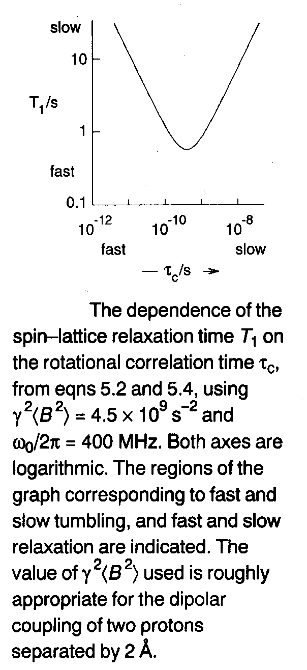
We have the information to predict how the spin-lattice relaxation rate varies with the rate of molecular motion. The graph to the right is significant.

It shows that J(ω0) is small for root-mean-square tumbling rate (i.e. τc-1) much smaller than ω0, or much larger than ω0, and reaches a maximum when τc-1 matches the resonance frequency (ω0τc = 1).

For rapidly tumbling molecules with ω0τc << 1, J(ω0) ≈ 2τc and the relaxation gets slower as the mean tumbling rate is increased (e.g. by raising the temperature). Conversely, slowly tumbling molecules have ω0τc >> 1 and J(w0) ≈ 2/ω02τc, so that the relaxation accelerates as the tumbling speeds up. The maximum relaxation rate (minimum T1) occurs ωοτc = 1, at which point J(ω0) = 1/ω0.

To decide whether a given molecule falls on the left or right of the T1 minimum, one needs to know τc. This is often not found easily (although can be approximated).

It can now be seen why rotational motion is important for most spin relaxation mechanisms – vibrations are usually much too fast to have a significant component at the relatively low frequencies involved in NMR. Modulation of intermolecular dipolar interactions by translational motion is also relatively inefficient because the couplings are generally weaker (larger average nuclear separation) than in the intramolecular case. Rotation, by contrast, occurs at roughly the right frequency, modulates intramolecular interactions, and so is near optimal for relaxation.

To see how spin-lattice relaxation depends on the local magnetic fields that cause it, we look at the predicted relaxation rate for the idealised random fields mechanism:

Where the spectral density has been discussed above and <B2> is the mean square value of the local fluctuating fields. Not surprisingly, stronger local fields lead to faster relaxation, other things being equal.

Spin-lattice relaxation rate of a pair of interacting nuclei should be proportional to r-6. T1’s are thus sensitive to the internuclear separations and hence molecule structure. Further, the mean square dipolar field produced by a spin S is proportional to the gyromagnetic ratio squared, so that the spin-lattice relaxation rate of a nearby spin I should be proportional to γΙ2γS2. A proton therefore relaxes a nearby 13C much less efficiently than a 1H at the same distance.

Nuclear spin relaxation is slow for two reasons. First, the local magnetic fields are generally rather feeble, and interact weakly with the nuclear spins. Second, the interactions must be rapidly modulated to be effective; and even when ω0τc = 1, the spectral density at the NMR frequency is small.

Spin-Spin Relaxation

Spin-Lattice relaxation is not the only way relaxation process affect NMR linewidths, and so it is useful to define a new parameter, the spin-spin relaxation time, T2 –

Where Δν is the linewidth associated with relaxation processes. T2 has a more fundamental interpretation, but for now we regard it as a linewidth parameter.

The second contribution to the linewidth, and hence T2, may be understood from the following argument. Imagine a disordered molecular solid in which all motions are frozen out. Every nucleus has several neighbours, to each of which it has a dipolar coupling. The NMR line of every spin is therefore split many times over by the dipolar interactions with neighbouring spins each with different r and θ. When this already complicated pattern is summed over all possible orientations of the molecules in the disordered solid, the result is a single, largely featureless peak with a width related to the root-mean-square dipolar interaction, which might be several kilohertz.

Quadrupolar Relaxation

A nucleus with a spin quantum number greater than ½ possess an electric quadrupole moment in addition to its magnetic dipole moment. One can think of this in terms of an ellipsoidal charge distribution in the nucleus with an excess of positive charge near the north and south poles and a corresponding depletion around the equator. Unlike electric dipoles – for example polar molecules HCl – electric quadrupoles do not interact with spatially uniform electric fields, but only with electric field gradients, a property that may be understood by regarding the nuclear quadrupole moment as two identical back-to-back electric dipoles.

The electric field gradient at a nucleus is a measure of the non-uniform distribution of local electronic charge: in sufficiently high symmetry environments – spherical, cubic, octahedral or tetrahedral – the electric field gradients generated by surrounding charges exactly cancel out, giving no net quadrupolar interaction. Nuclei in lower symmetry environments, however, experience non-zero electric field gradients which depend on the orientation of the molecule in the magnetic field of the NMR spectrometer. For example, two negative charges at a fixed distance from a quadrupolar nucleus have a more favourable Coulombic interaction when they are on the spin axis, i.e. close to the poles of the non-spherical nucleus, than on when they are in the equatorial plane. This anisotropic interaction, like the magnetic dipolar coupling, produces splittings in the NMR spectra of single crystals, and gives broad lines for powders and disordered solids. Quadrupolar interactions also cause spin relaxation when modulated by molecular tumbling.