Kinetics & Mechanism Notes

Basic Ideas

aA + bB → xX + yY

Molecularity, a wrt A and b wrt B (a+b+…)

Rate Equation:

Rate Constant:

Rate = k [A] α [B] β

Units – conc time-1/(concα concβ) → conc(1-(α+β)) time-1

i.e. 1st order → time -1, 2nd order → conc-1time-1 = dm3 mol-1s-1

How to Determine Order

3 methods:

Differential                 – if initial rates given.

Fractional Lives         – order only.

Integral                 – more than order to determine.

Need to isolate, e.g.

2NO → 2NO2

v = k[NO]2[O2]

Excess O2 → v = k’ [NO]2, where k’ = k[O2], i.e. becomes pseudo-2nd order in [NO].

 

Differential Methods –

One species / pseudo one species.

log (rate) = log k’ + α log [A]

(when rate = k’[A]α)

Plot a graph of log(rate) against log [A] – intercept k’, gradient α.

Fractional Lives –

1st order: τ1/2 = ln 2 / k                 (independent of concentration)

Else,

τ1/2 

i.e. zeroth order → Ao/2k, 2nd order → 1/kAo, etc.

Must remember that although the proportionality is valid for any fractional order, the constant will change between them.

Also worth remembering that if there’s not enough data, lower fractions e.g. ¼ lives can be used instead with the same result.

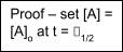
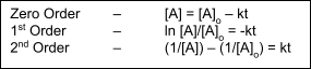
Integral Methods –

1st Order:

Activation Energies & Collision Theory

Increased temperature → k(T) increases (normally).

k = Ae-E/RT

(Arrhenius Equation)

→ ln k = ln A – EA/RT

Can have negative Activation Energies though, e.g.

           K1

NO + NO ⇌ (NO)2

                                                    k2

(NO)2 + O2 ⇌ 2NO2

Increase T → [dimer] falls, i.e. ↑T → ↓ rate. Basically, K1 drops much faster than k2 can increase.

Collision Theory of Reaction Rates

Collision Theory – simplest, and a theoretical rationalisation for the Arrhenius Equation. It seeks to predict the rate of a bimolecular elementary step:

A + B → products                v = k[A][B]

The rate of reaction is assumed to be equal to the collision frequency, ZAB, multiplied by the fraction of collisions having an energy greater than a critical energy Ec (the minimum energy required to react). The collision rate is given by the gas-kinetics result for hard-spheres:

The fraction of collisions that lead to reaction is assumed to have the form e-E/kT. The justification that is often given is that the Maxwell-Boltzmann distribution has the form:

where f(E)dE is the fraction of molecules with energies between E and E+dE. Integrating this expression from Ec to infinity gives the required expression.

Note: the apparent simplicity of this derivation is somewhat disingenuous for several reasons.

1. Conservation of momentum requires that only kinetic energy associated with the relative motion of A and B can be used for reaction. The one-dimensional Maxwell-Boltzmann distribution for relative velocity is not of the form above.
2. Molecules with a higher relative velocity collide more often. Thus the Maxwell-Boltzmann distribution needs to be weighted by the relative velocity.
3. Angular momentum needs to be conserved; unless the collision is head-on, only some of the kinetic energy of relative motion is available for reaction.

The collision theory expression is thus:

From the definition of the activation energy,

Ea = Ec + ½ RT                         (in molar terms)

Generally Ea >> RT, so the term ½ RT can be neglected.

Some Limitations of Collision Theory

• Calculated values of A ~ 1011-1012 dm3 mol-1 s-1 independent of the reaction, since A varies rather slowly with mass and temperature (A scales as √(T/m)).

Steric Factor, P, introduced to account for the difference between observed and calculated pre-exponential factors.

Limitation: except for a few special cases, there is no simple way of calculating P.

• For a reaction at equilibrium,

and

Collision Theory predicts the following relationship for the equilibrium constant K:

But from thermodynamics, , i.e. has entropy and enthalpy components. The entropy component has been lost in collision theory.

• For complicated molecules, measured values of k1 greatly exceed values calculated from collision theory because the energy stored in internal degrees of freedom (vibrations, internal rotations) have been ignored. Transition State Theory fixes this (see Reaction Dynamics Notes).

Measuring Rates of Reaction

1. Mixing – FAST. In situ generation.
2. Measuring – FLASH PHOTOLYSIS.

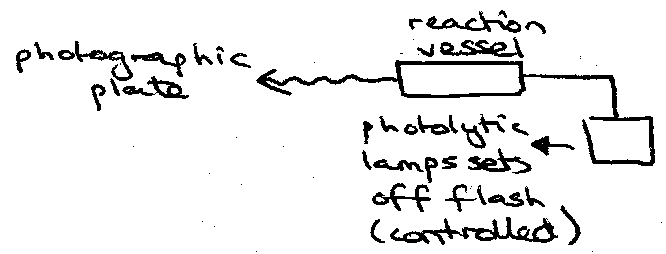
Flow Methods – (1ms to 1s) – no photochemical precursor.

Complex Reactions

The simplest complex reaction consists of two consecutive, irreversible elementary steps, e.g.

                                              k1     k2

A → B → C

If k2 >> k1, [B] is consumed as fast as it is produced and the equation for [C] reduces to:

                 k2 >> k1

The rate of production of [C] no longer depends on k2. The initial step is described as the rate determining step.

Conversely, if k1 >> k2 then all of [A] is rapidly converted to [B], which only slowly forms [C]. The integrated rate law for [C] is now independent of k1, except at the very beginning of the reaction:

                k1 >> k2

The second step is now rate determining.

For mechanisms that are only slightly more complicated, e.g.

                                                 k1     k2

A + B ⇌ C → D

                                                 k-1

it is generally impossible to find a solution to the differential equations in a closed form. One either has to integrate the differential equations numerically or resort to approximate methods.

Simple approximate solutions exist when (i) A, B and C are in equilibrium, and (ii) when C is a reactive intermediate.

Pre-equilibrium

The reaction scheme above occurs widely in chemical problems. If k-1 >> k2, A, B and C can be considered to be in an equilibrium that is barely perturbed by the slow leakage of [C] into product.

Keq = [C]/[A][B]

At equilibrium,

k-1[C] = k1[A][B]

For the reaction,

The reaction follows a second-order rate law with a composition rate constant as shown.

The pre-equilibrium assumption will not hold in the very early stages of the reaction while the equilibrium between A, B and C is being established.

Steady-State Approximation

The steady-state approximation (SSA) can be applied to reactive intermediates. More specifically, if the rate of change of the concentration of some intermediate, d[B]/dt is small compared to the rate of change of the concentrations of the reactants and products then we can set d[B]/dt equal to zero. As a general rule, if [B] << [reactants] throughout the reaction, the SSA will hold except at the very beginning of the reaction.

e.g. apply SSA to the simple consecutive scheme:

                                              k1     k2

A → B → C

The result of the SSA agrees with the full expression in the limit k2 >> k1:

Limiting cases for the reaction mechanism:

                                                          k1     k2

A + B ⇌ C → D

                                                 k-1

(i) k-1 << k2: consecutive irreversible reactions.

(ii) k-1 >> k2: pre-equilibrium.

(iii) k2, k-1 >> k1[A], k1[B] → d[C]/dt ~ 0: SSA can be applied to [C].

Chain Reactions

e.g. H2+Cl2

Cl2 → Cl + Cl                        [ initiation ]

Cl + H2 → HCl + H                [ propagation ]

H + Cl2 → HCl + Cl                [ propagation ]

Cl + Cl + M → Cl2 + M                [ termination ]

e.g. H2 + Br2

Br2 → Br + Br

Br + H2 → HBr + H

H + Br2 → HBr + Br        slows the reaction due to competition.

H + HBr → H2 + Br

Br + Br + M → Br2 + M

e.g. H2 + I2

I2 → I + I

I + H2 + I → 2HI        [ termolecular – not a chain reaction ]

I + H2 has a large EA → slow.

Branched-Chain Reactions

φ is the net branching factor.

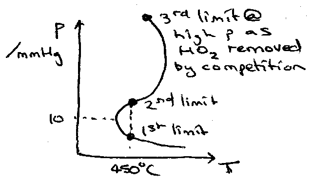
Hydrogen-Oxygen Reaction

H2 + O2 → OH + OH                [ initiation ]

OH + H2 → H2O + H                [ straight-chain ]

H + O2 → OH + O                [ branching ]

O + H2 → OH + O                [ branching ]        

H,OH,O + wall → loss                [ surface loss ]

H + O2 + M → HO2 + M                Rate Determining Step

HO2 + wall → loss                [ gas phase loss ]

Divide φ into branching term f and breaking term g.

φ = f – gwall - ggas

Unimolecular Reactions

The term “unimolecular reactions” is often used rather loosely to refer to gas-phase reactions that exhibit first-order kinetics and apparently involve only one chemical species. Examples include the isomerisation of cyclopropane:

And the decomposition of azomethane:

CH3N2CH3 → C2H6 + N2                v = kuni[CH3N2CH3]

The key question that arose in the early years of the century is how the molecules acquired sufficient energy to react, since the first-order kinetics appeared to preclude a bimolecular activation step. In 1922, Lindemann proposed the following mechanism:

                                                  k1

A + M ⇌ A* + M

                                                  k-1

                                                k2

A* → P

Where A* is an energised molecule and M is a collision partner that provides A with sufficient energy to react. Note that the Lindemann mechanism for decomposition reactions, is the reverse of the association reaction of radicals.

To determine the rate law for this mechanism, put A* in steady-state:

Comparing this equation with the experimental laws, one predicts that the rate “constant” kuni should not be a constant at all! At high pressures, however, k-1[M] >> k2 and the predicted rate law reduces to the experimental rate law with a rate constant k∞ = k1k2/k-1. At low pressures where k-1[M] << k2, the predicted rate law becomes second-order, reflecting the bimolecular nature of the activation step which has now become rate-determining. The change over the second-order kinetics at low pressures was first observed by Ramsperger in 1927.

Lindemann mechanism predicts that a double reciprocal plot of kuni-1 vs. [A]-1 should be linear.

While the essential activation process embodied in the Lindemann mechanism is generally accepted, this model does have a number of serious failings. See Reaction Dynamics Notes for more sophisticated models.

Enzyme Kinetics

The rate of enzymatic reactions is often found empirically to follow the Michaelis-Menton Equation:

where S is the substrate and KM is called the Michaelis constant. The maximum rate, vmax, is found to be linearly proportional to the total concentration of enzyme:

vmax = kcat[E]o

kcat is the turnover number (maximum number of molecules of substrate that each molecule of enzyme can “turn over” per second). Simplest mechanism consistent with this rate law:

                

E + S ⇌ ES                                ES → P + E

   

E = enzyme, S = substrate, ES = enzyme-substrate complex, P = product.

Apply SSA to ES:

          Rate of Reaction:        

Expressing the (unknown) concentration of free enzyme, [E], in terms of the total concentration of enzyme [E]o = [E] + [ES] yields the rate law:

This rate law has the same form as the Michaelis-Menton Equation if we identify kcat with k2 and KM with (k2+k-1)/k1.

Several standard plots for obtaining vmax and KM from kinetic data on enzymatic reactions, the simplest being a double reciprocal or Lineweaver-Burke plot. Usually the initial rate method is employed since it avoids any complications resulting from reactions of the products.