Electronic Spectroscopy Notes

Each electronic state has its characteristic potential energy curve which supports its own set of vibrational and rotational levels → change of associated vibrational and rotational quantum numbers.

Term Symbols

• Left superscript S = spin multiplicity.
• Capital Greek letter is the electronic angular momentum Λ along the molecular axis.
• Right subscript gives the inversion symmetry (g is even, u is odd).
• Right superscript + or – gives symmetry of Σ states to reflection in a plane containing the molecular axis.

Designation of Diatomic Energy Levels

Atoms – couple angular momenta of electrons to label states. Same for molecules. Filled orbitals have no resultant spin/orbital angular momentum.

Spin Angular Momentum, Σ

• closed shell, Σ = 0, multiplicity = 1 (singlet)
• one unpaired electron, Σ = ½, multiplicity = 2 (doublet)

Orbital Angular Momentum, Λ

• σ, Λ = 0
• π, Λ = 1. Degenerate π → π+ and π- (+1/-1)

Term Symbols – as for atoms.

Λ → Σ, Π, Δ

2Σ+1Λ

e.g. closed shell = 1Σ.

Also, g/u subscript for homonuclear diatomics (inversion centre).

+/- superscript for symmetry wrt plane through nuclei.

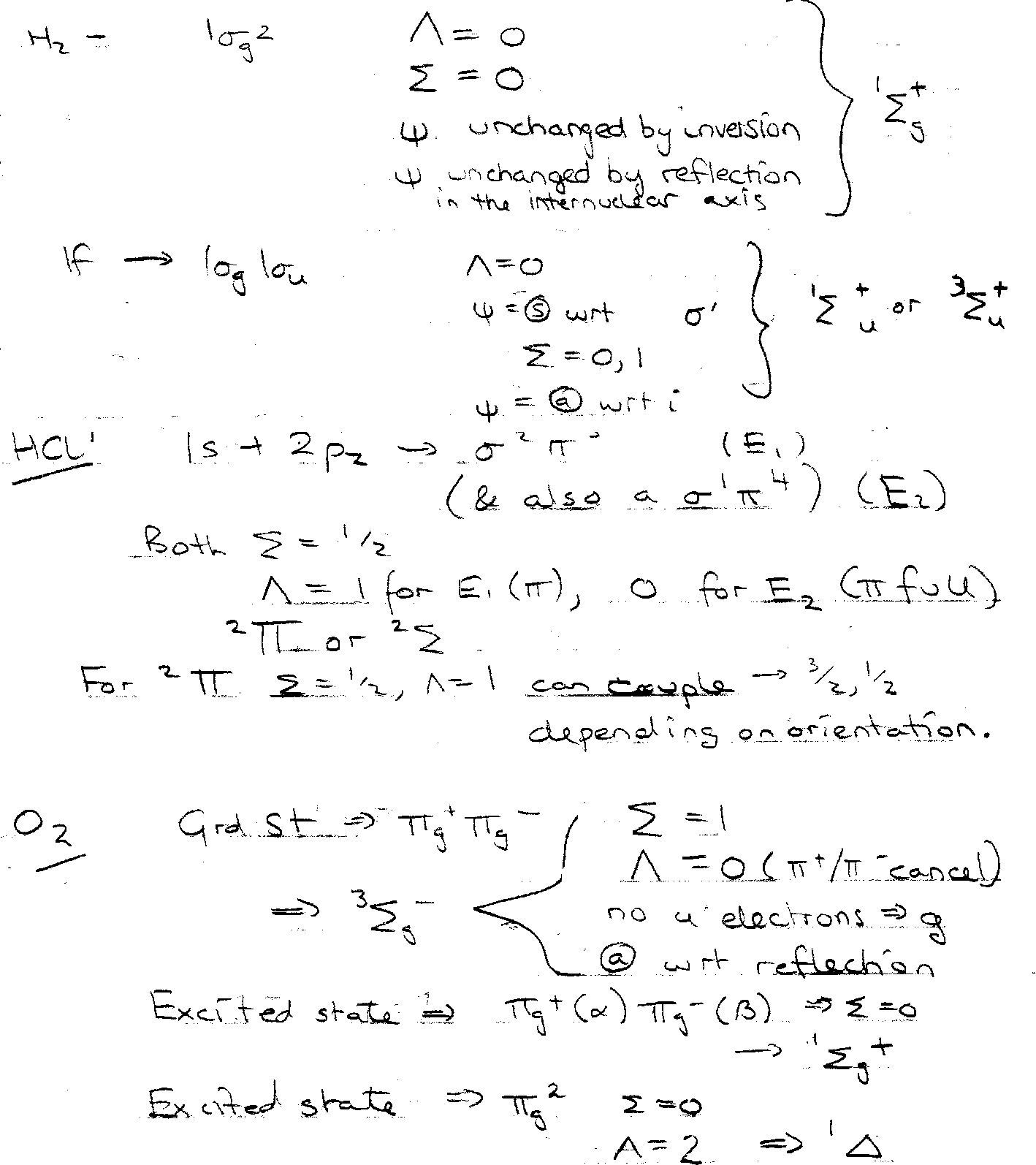
H2 / N2 → 1Σg+

O2 → 3Σg-.

Examples:

Each electronic state has vibrational and rotational fine structure.

Electronic Hamiltonian

Wel = Tel + V

Tel =

Helψel = Eelψel

No known solution for ψel in a simple form. Need to know symmetry properties.

Orbital Approximation –

Nuclear-Nuclear term is constant (constant r).

One electron terms – KE and nucleus-electron attraction.

2 electrons in e-e repulsion (cannot be solved).

Ignoring e-e repulsion for the moment, we have Hel ≈ Helo.

Solving this independent electron form gives the orbitals we are used to.

For molecules, LCAO is used.

Vibrational and Rotational Structure –

The motions of electrons in a molecule takes place on a very short timescale (10-15s) for the duration of which the nuclei are fixed.

Vibration – 10-13s.                                Rotation – 10-11s.

Vibrational Energy Levels:

G(v) = Evib/hc = (v+½)ωe - (v+½)2ωexe + …

Rotational Energy Levels:

F(J) = Erot/hc = BvJ(J+1) – DvJ2(J+1)2 + …

Selection Rules

Electronic - < i | μ | f > ≠ 0, where μ is the components of the electric dipole.

Neglect S-O coupling,

ΔΣ = 0.                [ can deviate when S-O coupling begins to be significant ]

ΔΛ = 0,±1

u↔g only.

+↔+ / - ↔ - only (for Σ→Σ)

For the vibrational part in absorption, emission and photoelectron spectra:

1. Totally symmetric vibrations can be excited (includes all diatomic vibrations).
2. Δv is restricted only by the Franck-Condon Principle (see below). The relative intensity vi → vf is proportional to |<vf|vi>|2.

For the rotational part in absorption and emission:

• In Σ↔Σ transitions, ΔJ = ±1.
• In Σ↔Π transitions, ΔJ = 0,±1.
• distinguish between parallel (ΔJ = ±1) and perpendicular (ΔJ = 0,±1).

Determination of Molecular Properties –

From Spectra (shape of PE curve for each electronic state) – excitation energy, bond lengths, vibrational frequency, dissociation energy.

Intensities given by:

This gives rise to the Franck-Condon Principle – see transitions to vibrational states with large overlap with vibrational wavefunctions for the initial state.

i.e. transition with maximum vibrational overlap is the “vertical transition”, i.e. transition with stationary nuclei.

This is also true in photoelectron spectroscopy (except the upper state is now ionic). Successive Ionisation potentials ≈ energy of orbitals from which the electron is removed.

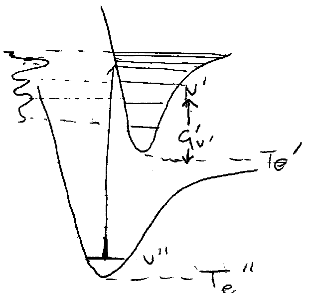
Franck-Condon Principle:

v’’ → v’ bands.

If the potential curves are similar, in particular if re’’ ≈ re’, then the (0,0) band dominates the spectrum (best overlap v’’=0 → v’=0).

Most favoured can be found by drawing from r = re’’ (minimum) upwards to where it meets the excited state’s curve.

If re’’ = re’, states either side will also have significant intensity.

The progression is the run of adjacent vibrational bands seen when the equilibrium bond length changes on excitation. Usually looks like:

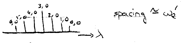
If bond length changes, many vibrational levels are seen, so ΔG(v) can be plotted against v in the upper state (Birge-Sponer plot). One intercept is ωe, the other gives the vibrational quantum number at the dissociation limit.

The dissociation energy can be estimated:

• By putting vdis into the vibrational energy equation,
• As area under the line (which will not generally be straight all along it),
• As ωe2/(4ωexe), which assumes a straight line.

Rotational (Branch) Structure –

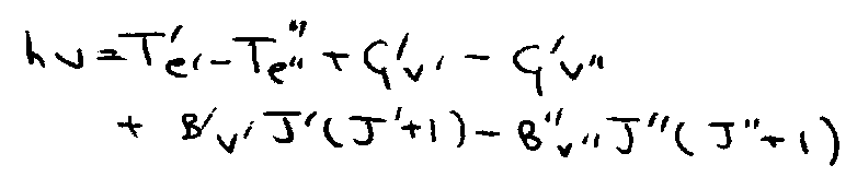
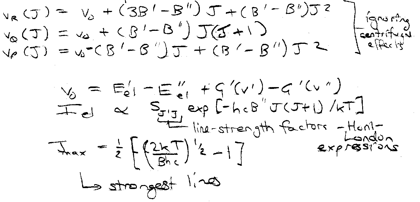
Transitions at frequencies –

Note rotational constant depends on vibrational state as B’v’ = B’e - α(v’+½).

Because of very different bond lengths in Ground and Excited State, (B’-B’’) may be large. This leads to formation of “band heads” where line separation gets very small.

To extract rotational constants we use combination-differences (as for vib-rot) to find bond lengths.

Each vibrational band consists of a number of rotational lines. Similar to those found in vib-rot spectra.

Same expressions, but can differ greatly from vib-rot spectrum. This is due to very different B values.

In electronic transitions the change in bond length is often big, so there can be a big difference in B. This makes the lines in one branch, P or R, close up until they overlap forming a “head” where intensity is concentrated, while lines in the other branch spread out. If the bond lengthens on excitation (B’’>B’) the head is in the R branch (towards violet) and the “tail” is to the red. If the bond shortens, the head is to the red and tail to the violet. So the direction of bond length change can be seen from band shapes even if rotation is not resolved.

If absorption / emission spectra is shown, and absorption lines don’t have matching emission lines, then predissociation is seen.

B’ < B’’

• infrared → R branch close lines slightly, while P branch spread out with ↑J.
• electronic → R branch spacing → 0, and doubles back at 0. Spacing – several lines in close proximity (a branch head).

J value at branch head given by:

This is most common state, as bond is usually longer in the upper electronic state.

Rotational structure spreads out to lower v (red degraded).

If B’ > B’’ instead, the branch head is in P. By the same method,

.Extracting full information from rotational structure is achieved in the same way as vib-rot – use Combination Differences and assigned rotational quantum numbers.

Dissociation & Predissociation

Can absorb enough radiation to break the bond and dissociate the molecule (Do’’ measured from v’’=0). This is less likely than → v’, but still occurs.

Other things that can happen with excitation:

• dissociation
• fluorescence, e.g. v = 4 re-emits radiation ↓v’’.
• ↓v’=0 by collisional relaxation, then ↓v’’.
• radiationless transition, v’=0 → v’’= a high number. Slight possibility, and more likely in condensed phase.

Dissociation occurs if absorbed energy takes above required v’ state (no competing processes).

Eex = (Do’ + v00 – Do’’)

(Excitation Energy of A* state product – A = upper state).

Anharmonicity → vibrational spacing decreases as v increases.

Dissociation limit → spacing → 0.

G(v’) = (v’+½)ωe’ - (v’+½)2ωexe’ for lower vibrational levels.

Hence, ΔG(v’) → 0 at (vL’+½) = ωe’/2ωexe’.

Energy at this point = ωe’2/4ωexe’ above minimum of A state curve.

Formula corresponds to a Morse Potential.

The formula is used graphically: ΔG(v’) vs. v+½, and area under = energy required to dissociate. This is a Birge-Sponer extrapolation (estimate).

• hvv’v’’ = T’e’ – T’’e’’ + G’v’ – G’’v’’
• (Usually v’’ = 0 in absorption).
• Plot ΔG’v’+1/2 = hv(v’+1)v’’ – hvv’v’’
• Difference of successive lines vs. v’ + ½ → straight line.

2 weaknesses:

• extrapolate so exaggerate errors in measurement of band heads near dissociation limit.
• Morse Formula less reliable as v increases, so curve bends downwards instead of straight line.

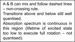
Predissociation – (collapse of fine structure).

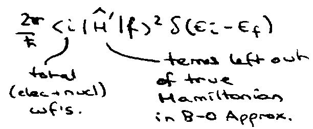
Upon excitation, excited molecule is formed in the bound state. This mixes with the continuum states so that the initial state has only a finite lifetime.

The mixing occurs because the adiabatic states are only approximate eigenstates – due to B-O Approximation.

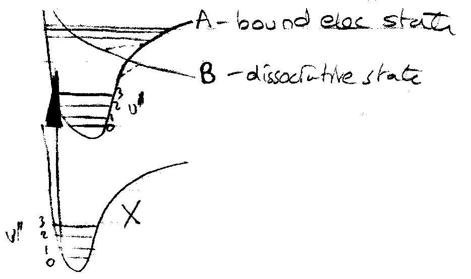
• Rotation band head disappears.
• Vibration band head appears “fuzzy”.

Result is sharp peaks for v’ = 0 … 3, then fuzzy, then resume sharp peaks.

Normal dissociation occurs at high quantum numbers.

Crossing point dissociation therefore equals predissociation.

Relaxation Rate is given by:

Also get,

Intersystem Crossing – due to S-O Coupling.

Internal Conversion – Also Born-Oppenheimer breakdown.